Population models

In this chapter we discuss models for populations data: observations from a set of individuals sampled from a population. The data is characterized by one or more observations for each individual. We are mainly interested in parametric models and estimations of the random parameters.

Problem formulation

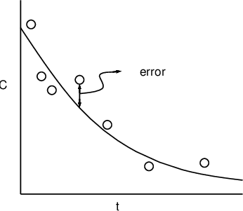
Individuals in a sample of size $N$ are different due to fixed and/or random effects, manifested as individual parameters $\phi_i$ (clearance, volume of distribution, etc), $i=1,\dots,N$. For a general formulation for mixed-effects model we consider a function $f()$ of known quantities $x_{ij}$ (doses, covariates, time, etc) and unknown parameters $\phi_i$ to describe observations $y_{ij}$ (plasma concentration, drug effect, etc). $f()$ is sometimes referred to as structure model. Since in reality $f(x_{ij}, \phi_i)$ cannot account for all the variability of $y_{ij}$, we additively complement it with a residual error term.

Longitudinal concentration ($y_{ij}=C$) data points and error term in an exponential model.

In summary

\begin{equation} y_{ij} = f(x_{ij}, \phi_i) + h(x_{ij}, \phi_i)\epsilon_{ij}. \end{equation}

Subscript $ij$, $j=1\dots,N_i$ denotes observation $j$ for individual $i$. Then total number of observations in a data set is $N_{\text{obs}}=\sum_iN_i$. In general individuals do not have the same number of observations: $N_i\ne N_k$ when $i\ne k$.
The term "nonlinear" in "nonlinear mixed-effects model" is related to $f()$ being nonlinear with respect to its arguments.
For the residual error, We assume that $\epsilon_{ij}$ follows a multivariate normal distribution ¹,

$$ \epsilon_{ij} \sim \text{MultiNormal}(0, \Sigma). $$ The covariance matrix $\Sigma$ is represented in NONMEM by reserved variable SIGMA. This implies $\epsilon_{ij}$ can be a vector (see below). We also assume $\epsilon_{ij}$ are independent from $\epsilon_{kl}$ when $(i,j)\ne (k, l)$. We use (matrix) function $h()$ to adjust $\epsilon$ so that the residual error in general has variance $h\Sigma h^T$. Consider the following examples.

$\epsilon$ is a scalar and $h()\equiv 1$ a constant. It represents homoscedastic residual error: all the observations $y_{ij}$ share a same normally distributed residual error. This is sometimes referred to as additive residual error model.

Additive residual error model.
$\epsilon$ is a scalar and $h(x_{ij},\phi_i)=f(x_{ij},\phi_i)^{\xi}$. It represents the power error model. When $\xi=1$ it becomes the proportional error model in which the residual error variance is proportional to the squared prediction;

Proportional residual error model.
$\epsilon$ is a 2-vector and $h(x_{ij}, \phi_i)=[f(x_{ij}, \phi_i), 1]^T$. It combines the additive and proportional model, equivalent to $$ y_{ij} = f(x_{ij}, \phi_i) + f(x_{ij}, \phi_i)\epsilon_{ij}^{(1)} + \epsilon_{ij}^{(2)}, $$ $$ \epsilon_{ij}^{(1)} \sim \mathcal{N}(0, \upsilon_{11}), $$ $$ \epsilon_{ij}^{(2)} \sim \mathcal{N}(0, \upsilon_{22}). $$ The variances $\upsilon_{11}$ and $\upsilon_{22}$ are the diagonal elements of $\Sigma$.
$\epsilon$, $y_{ij}$ and $f()$ are 2-vectors, and $h()$ a $2\times 2$ matrix. It represents a multivariate model. This could be the case when observations are the plasma concentrations in both central and peripheral compartments, or from two tissues/organs in a physiologically based PK (PBPK) model.

NONMEM provides control record $ERROR to specify the residual error $h(x_{ij}, \phi_i)\epsilon_{ij}$.

Sometimes we use the vectorized representation for subject i
\begin{equation} y_i=f(x_i, \phi_i) + h(x_i, \phi_i)\epsilon_i. \end{equation}
For example, for the above combine error model, $y_i$ and $f()$ would be a $N_i$-vector, $h()$ a $N_i\times 2N_i$ matrix, and $\epsilon_i$ a $2N_i$-vector.

Next we describe the models for $\phi_i$. We assume $\phi_i$ has a "typical" value $\bar{\phi}_i=\mu(z_i, \theta)$. By "typical" we mean that the value is the same for individuals with same covariates $z_{i}$, e.g. weight and height. We then assume $\phi_i$ deviates $\bar{\phi}_i$ by a random perturbation $\eta_i$:

\begin{equation} \phi_{i} = \mu(z_{i}, \theta) + \eta_{i}. \end{equation}

We refer $z_i$ as the fixed effects, and $\theta$ the fixed effect parameters ². NONMEM uses reserved variable THETA for $\theta$ ³. We refer $\eta_i$ as the random effects parameters. NONMEM uses reserved variable ETA for $\eta$. In general $\theta$, $\phi_i$, and $\eta_i$ are vectors. NONMEM output use PHI for $\phi_i$.

A nonlinear $\mu()$ contributes further to the nonliearity of the problem.
NONMEM assumes all $\eta_i$'s follow a multivariate normal distribution ¹, $$ \eta_i \sim \text{MultiNormal}(0, \Omega). $$ NONMEM uses reserved variable OMEGA for the covariance matrix $\Omega$.

In some of NONMEM's solution algorithms the above $\mu() + \eta$ pattern can improve efficiency. See MU referencing.

NONMEM refers the random effect with $\phi$ (or equivalently $\eta$) as the first-level, and the randomness due to $\epsilon$ the second-level. By definition the residual error's variance-covariance structure, $h(x,\phi)\epsilon$, contains both levels of random effects, as $\phi$ (or $\eta$) interacts with $\epsilon$ in the residual error term. This behavior is accounted for in NONMEM's estimation methods through option "INTERACTION". By default the INTERACTION is not activated, and the estimation is based on residual error $h(x, \phi|_{\eta=0})\epsilon$. We recommend always use INTERACTION.

Covariate models

In NONMEM guides the models for $\mu()$ are called structure parameter models. Here to avoid confusion with the model for $f()$, we use the term "covariate models", and discuss a few common ones in PK applications. Assume $\phi$ has clearance CL as one of its elements, then we use $\tilde{\text{CL}_i}=\mu(z_i, \theta)$ for TVCL ⁴, the "typical value" of CL. In NONMEM the above equation for $\phi$, i.e. the association of $\theta$, $\eta$, and $z$, are encoded in control record $PK.

Linear (additive) models

The simplest form of $\mu()$ is its being linearly related to $\theta$. For example, if CL is the sum of renal and non-renal components (CL_ren and CL_met, respectively), and CL_ren is believed to be proportional to renal function (RF) as described according to a standard formula involving covariates in $z$: age (AGE), serum creatinine (SECR), and weight (WT), then one might consider the following model (we omit subscript $i$ to avoid clutter).

$$ \tilde{\text{CL}}_{\text{met}} = \theta_1 \text{WT}, $$ $$ \text{RF}=\text{WT}\frac{1.66-0.011\text{AGE}}{\text{SECR}}, $$ $$ \tilde{\text{CL}}_{\text{ren}} = \theta_4 \text{RF}, $$ $$ \tilde{\text{CL}} = \tilde{\text{CL}}_{\text{ren}} + \tilde{\text{CL}}_{\text{met}}. $$ Despite RF being a nonlinear function of covariates, the above model shows a linear $\mu$ with respect to $\theta$, as (we use $\cdot$ for inner product) $$ \tilde{\text{CL}} = (\text{WT}, \text{RF}) \cdot (\theta_1, \theta_4). $$

Multiplicative model

Multiplicative models are linear models on a logarithmic scale. For example, if patients covering a very wide range of weights are studied, metabolic clearance might vary with weight, but not linearly. Then instead of modeling them linearly, we assume

$$ \log(\tilde{\text{CL}}_{\text{met}}) = \theta_1 + \theta_2\log(\text{WT}), $$ equivalently ⁵ $$ \tilde{\text{CL}}_{\text{met}} = \theta_1\text{WT}^{\theta_2}. $$ Note that the two sets of $\theta$'s are not the same, but since they are unknown parameters we can transform them and fit either set in a model. This reparameterization is common in statistical modeling.

Saturation Models

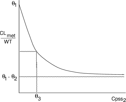
A useful model for processes reaching a maximum is a hyperbolic model. For example, if a second drug, (whose steady-state plasma concentration, Cpss_2 is known and given in the data set), is present in some individuals and it is believed to be an inhibitor of the metabolism of the study drug, one might consider

$$ \tilde{\text{CL}}_{\text{met}}=\text{WT} \left(\theta_1-\frac{\theta_2 \text{Cpss}_2}{\theta_3 + \text{Cpss}_2}\right) $$

The relationshiup is shown in figure below. The inhibition is expressed by the ratio occurring within the brackets and is a concave hyperbola, asymptoting to a maximum value equal to $\theta_2$. It is identical in form to the Michaelis-Menten model.

Indicator variables

Assume a binary variable HF documents the clinical condition of heart failure as "present" (HF=0) or "absent" (HF=1). To model heart failure affected CL_met, we do ⁵ $$ \tilde{\text{CL}}_\text{met} = (\theta_1 - \theta_2\text{HF})\text{WT}. $$ See details in "Cookbook: Indicator variables".

Population random effects models

Under NONMEM nomenclature, there are two levels of random effects, $\eta$ and $\epsilon$:

$\eta$ in the parameter model accounts for the inter-individual variability in $\phi$ that is not explained by $\mu(z_i, \theta)$;
$\epsilon$ accounts for the intra-individual variability that is not explained by $f(x_{ij}, \phi_i)$, thus formulates the error model.

The interindividual variability can arise from

the approximate nature of $\mu()$ to express the relation between covariates $z$ and individual parameters $\phi$;
the covariates $z$ contain measurement error.

The intraindividual variability can arise from

the approximate nature of the structure model $f()$;
observed quantities $x$ contain measurement error;
the pharmacokinetic responses $y$ contain measurement error (assay error).

Models for Interindividual variability

NONMEM uses $\eta$ to describe interindividual variability. Its covariance matrix $\Omega$ is symmetric and positive-semidefinite. NONMEM utilizes the symmetry so that only the lower triangular elements are used to specifiy OMEGA. For example, in a two-compartment model we can have $\eta=(\eta_{k10}, \eta_{k12}, \eta_{k21})$ for the elimination and transfer coefficients. Then $\Omega$ will be a 3x3 matrix but OMEGA contains only 6 elements, $$ \omega_{11}=\text{var}(\eta_{k10}),\quad \omega_{22}=\text{var}(\eta_{k12}),\quad \omega_{33}=\text{var}(\eta_{k21}) $$ for diagonal, and $$ \omega_{21}=\text{cov}(\eta_{k10}, \eta_{k12}), \quad \omega_{31}=\text{cov}(\eta_{k10}, \eta_{k21}), \quad \omega_{23}=\text{cov}(\eta_{k12}, \eta_{k21}) $$ for off-diagonal.

Additive model

An additive model, for example for volumn of distribution V:

$$ \text{V}=\tilde{\text{V}}+\eta $$

leads to unit-dependent $\omega$, as changing the unit of V will cause $\eta$ to change, so does its variance.

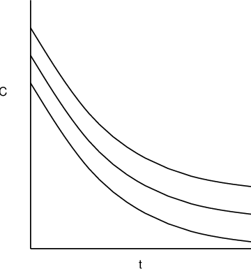
Multiplicative model

Also known as Constant Coefficient of Variation (CCV) model or proportional error model, a multiplicative model such as $$ \text{V}=\tilde{\text{V}}(1+\eta) $$ does not change $\omega$ when unit of V is alterered.

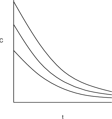
Exponential model

Exponential model is additive model on log scale. $$ \log(\text{V}) = \log(\tilde{\text{V}}) + \eta\quad \rightarrow\quad \text{V} = \tilde{\text{V}}\exp(\eta). $$ It does not change $\omega$ when unit of V is alterered.

Generalized formulation

Let us consider the following example. A study involves both patients in the intensive care unit (ICU) and in the non-acute care units. One could postulate that ICU patients have higher variability in kinetics such as metabolic clearance of drug due to unmeasured factors. For example, their hepatic function could vary greatly. Even though the variation is actually due to a potentially measurable fixed effect (hepatic function), when such information is not available, $\eta$ must account for the difference in variability in the two grups. One approach to do this is through indicator variable ICU: ICU=1 for ICU patients and ICU=0 otherwise, and metabolic clearance model ⁶

$$ \text{CL}_{\text{met}}= \tilde{\text{CL}}_{\text{met}} + (1-\text{ICU})\eta_1+\text{ICU}\eta_2, $$

in addition to renal clearance model

$$ \text{CL}_{\text{ren}}= \tilde{\text{CL}}_{\text{ren}}(1 + \eta_3). $$

Thus here $\phi$ (corresponding to CL here), is associated to more than one $\eta$'s ($\eta$_1-3 here), and not in the form of $\phi=\mu+\eta$. Another example where the additive form for $\eta$ is not applicable is when $\phi$ is associated with $\eta$ nonlinearly.

Hence we want to generalize the parameter model, so that ⁷

$$ \phi_i=\mu(z_i, \theta, \eta_i), $$ and we allow the dimention of $\phi_i$ and $\eta_i$ to be different.

Population mixed effects model

In summary, the population mixed effects model in NONMEM has the following general form.

\begin{equation} y_{ij} = f(x_{ij}, \phi_i) + h(x_{ij}, \phi)\epsilon_{ij}, \end{equation} \begin{equation} \phi_i = \mu(z_{i}, \theta, \eta_i). \end{equation}

In NONMEM we use "control records" to specify the above model. The $PRED control record can be used for general modeling, but for PK problems more often we use NONMEM's built-in models.

Control record $SUBROUTINES specifies $f()$. When $f()$ is the solution of a general nonlinear differential equation system, control record $DES, $AES, and $MODEL are used to describe the RHS.
Control record $PK specifies $\mu()$.
Control record $ERROR specifies $h()\epsilon$.
Control record $THETA, $OMEGA, $SIGMA specify the initial estimate and constraints of $\theta$, $\Omega$, and $\Sigma$, respectively.

All the mentioned control records will be discussed in the next part of the guide.

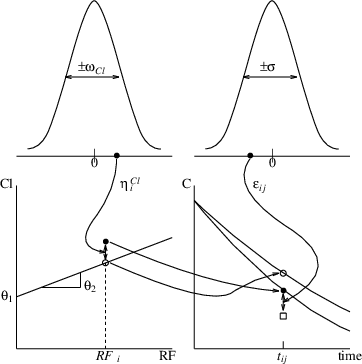
To express PK models in the above form, consider the example of one-compartment model with dose at the central compartment. $$ y_{ij}=\frac{D}{\text{V}_i}\exp\left(-\frac{\text{CL}_i}{\text{V}_i}t_{ij} \right) + \epsilon_{ij} $$

$$ \text{CL}_i=\theta_1 + \theta_2\text{RF}_i + \eta_i, \quad \text{V}_i=\theta_3 $$ Here we have $x_{ij}=(D, t_{ij})^T$ for dose, $z_i=\text{RF}_i$ for the covariate of certain measurement of renal function. The model assumes an interindividual variability for the clearance but not for the volume of distribution. Thus the $\eta$ is a scalar. Then we have $$ y_{ij}=f((D, t)^T, \phi_i=(\text{CL}_i, \text{V}_i)^T), $$ $$ \phi_i=(\text{CL}_i, \text{V}_i)^T=\mu(z_i=\text{RF}_i, \theta=(\theta_1, \theta_2, \theta_3)^T, \eta_i) =(\theta_1 + \theta_2\text{RF}_i + \eta_i, \theta_3)^T. $$ Note that the structure model $f()$ is a scalar function (for concentration), $\mu$ is a 2-vector function for $\text{CL}$ and $\text{V}$, $\theta$ is a 3-vector, and both $\Omega=(\omega_{\text{CL}}^2)$ and $\Sigma=(\sigma^2)$ are $1\times 1$ matrices. Figure below shows the relationship of the fixed and random effects

Random and fixed effects influence observation C from the population point of view.

In this document we use symbol $\sim$ to indicate a distribution statement. This is common in statistical literature.

The nomenclature can be confusing in statistical literature, as often $\theta$ is also called the "fixed effects", and the value of $\theta$ "fixed effects size". In this document we try to make the context clear whenever those terms are used.

Later on we will discuss situations when not all $\theta$'s are associated with $\mu$ or $\eta$ in this way.

⁴

Prepending "TV" to a quantity name is a common practice, but note "TVCL" is not a reserved name in NONMEM.

⁵

Heart failure is expected to decrease metabolic clearance. Thus using a minus sign here implies $\theta_2$ is assumed positive.

⁶

To avoid clutter here we use subscript for different $\eta$ for a same subject instead of subject ID.

⁷

Here the subscript is for subject ID. We hope the context is clear when we use the subscript differently.